Argos: User Documentation

Overview

Argos comes with four main components:

• Capture tool for capturing video with camera, or for extracting parts of an existing video.

• Tracking tool for automatically tracking animals in videos using either classical object segmentation or a neural net.

• Annotation tool for creating dataset to train the neural net for the Tracking tool.

• Review tool for manually reviewing and correcting the automatically detected tracks.

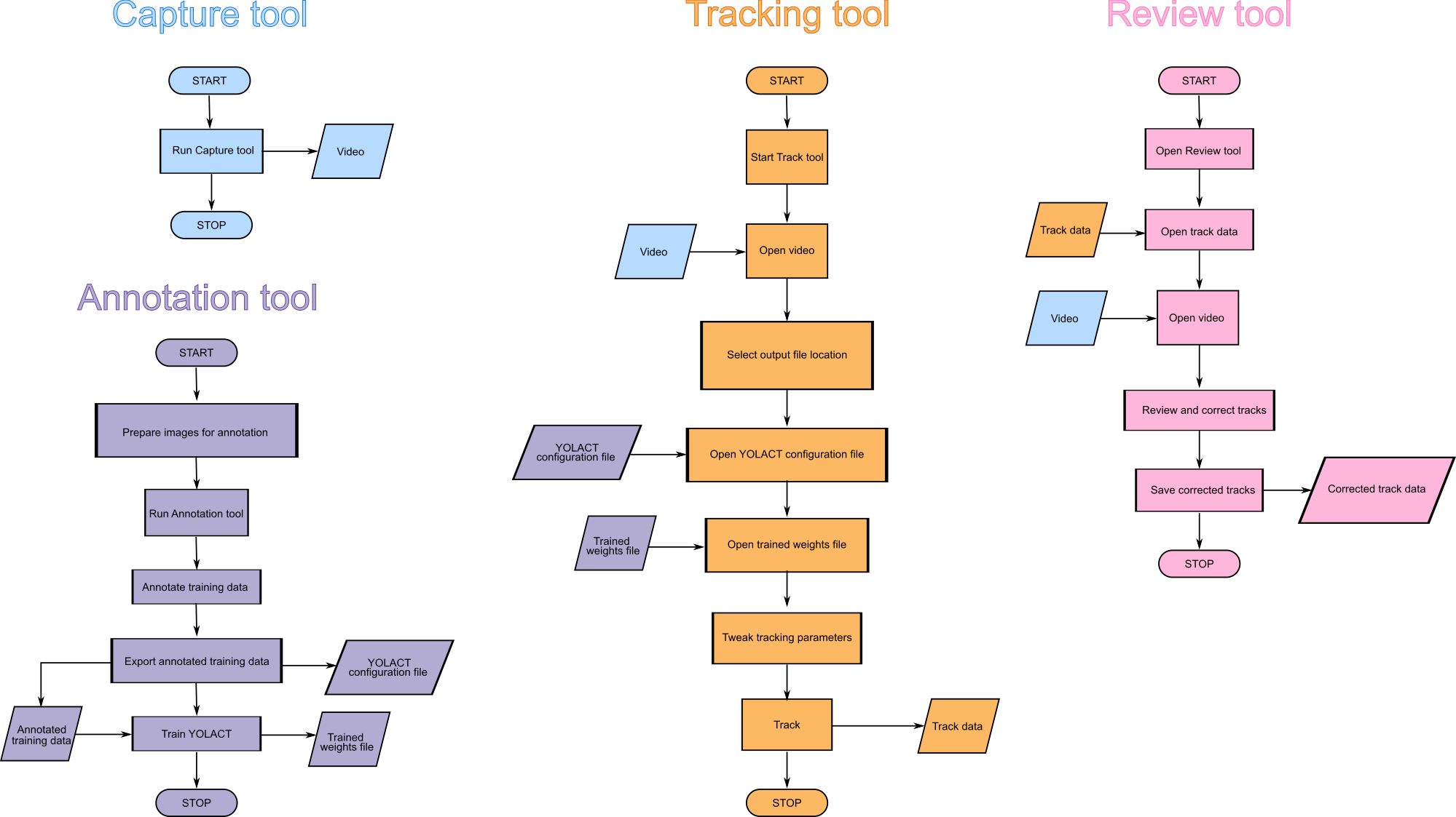
Fig. 1 Flow charts showing how to work with the four tools in Argos.

Capture or process video

Usage:

python -m argos.capture -i 0 -o myvideo_motion_cap.avi

To see a list of all options try python -m argos.capture -h

The above command will take a snapshot with the default camera on your computer and ask you to select the region of interest. Click your left mouse button on one corner of the region of interest and drag to draw a rectangle. Press Enter key when done (you may need to press it twice). If you want to change the selection, or moved the camera to adjust focus or frame, press C on the keyboard to update the image and draw the ROI again. Press Enter to start recording. This will create two files, myvideo_motion_cap.avi containing the recorded video and myvideo_motion_cap.avi.csv with the timestamp of each frame.

argos.capture is a simple tool to capture video along with timestamp for each frame using a camera. It can also be used for recording videos only when some movement is detected. When applied to a pre-recorded video file, enabling motion-based capture will keep only those frames between which significant movement has been detected.

What is significant movement?

• The movement detection works by first converting the image into gray-scale and blurring it to make it smooth. The size of the Gaussian kernel used for blurring is specified by the --kernel_width parameter.

• Next, this blurred grayscale image is thresholded with threshold value specified by the --threshold parameter.

• The resulting binary frame is compared with the blurred and thresholded version of the last saved frame. If there is any patch of change bigger than --min_area pixels, then this is considered significant motion.

These parameters will depend on the resolution of the captured video, lighting, size of animals etc. One can optimize the parameters by trial and error. A starting point could be checking the size of the animals in pixels and pass a fraction of that as --min_area.

Not all video formats are available on all platforms. The default is MJPG with AVI as container, which is supported natively by OpenCV.

If you need high compression, X264 is a good option. Saving in X264 format requires H.264 library, which can be installed as follows:

• On Linux: conda install -c anaconda openh264

• On Windows: download released binary from here: https://github.com/cisco/openh264/releases and save them in your library path.

Examples

1. Read video from file myvideo.mpg and save output in myvideo_motion_cap.avi in DIVX format. The -m --threshold=20 -a 10 part tells the program to detect any movement such that more than 10 contiguous pixels have changed in the frame thresholded at 20:

   python -m argos.capture -i myvideo.mpg -o myvideo_motion_cap.avi  \\
   --format=DIVX -m --threshold=20 -a 10
   

The recording will stop when the user presses Escape or Q key.

2. Record from camera# 0 into the file myvideo_motion_cap.avi:

   python -m argos.capture -i 0 -o myvideo_motion_cap.avi
   

3. Record from camera# 0 for 24 hours, saving every 10,000 frames into a separate file:

   python -m argos.capture -i 0 -o myvideo_motion_cap.avi \\
   --duration=24:00:00 --max_frames=10000
   

   This will produce files with names myvideo_motion_cap_000.avi, myvideo_motion_cap_001.avi, etc. along with the timestamps in files named myvideo_motion_cap_000.avi.csv, myvideo_motion_cap_001.avi.csv. The user can stop recording at any time by pressing Escape or Q key.

4. Record a frame every 3 seconds:

   python -m argos.capture -i 0 -o myvideo_motion_cap.avi --interval=3.0
   

Common problem

When trying to use H264 format for saving video, you may see the following error:

Creating output file video_filename.mp4
OpenCV: FFMPEG: tag 0x34363248/'H264' is not supported with codec id 27 and
format \'mp4 / MP4 (MPEG-4 Part 14)\'
OpenCV: FFMPEG: fallback to use tag 0x31637661/\'avc1\'

        OpenH264 Video Codec provided by Cisco Systems, Inc.

Solution: Use .avi instead of .mp4 extension when specifying output filename.

Annotate: Generate training data for YOLACT

Usage:

python -m argos.annotate

This program helps you annotate a set of images and export the images and annotation in a way that YOLACT can process for training. Note that this is for a single category of objects.

Preparation

Create a folder and copy all the images you want to annotate into it.

If you have videos instead, you can extract some video frames using File->Extract frames from video in the menu.

There are many other programs, including most video players, which allow extracting individual frames from a video if you need more control.

Upon startup the program will prompt you to choose the folder containing the images to be annotated. Browse to the desired image folder. All the images should be directly in this folder, no subfolders.

Annotate new images

After you select the image folder, the annotator will show you the main window, with an empty display like below.

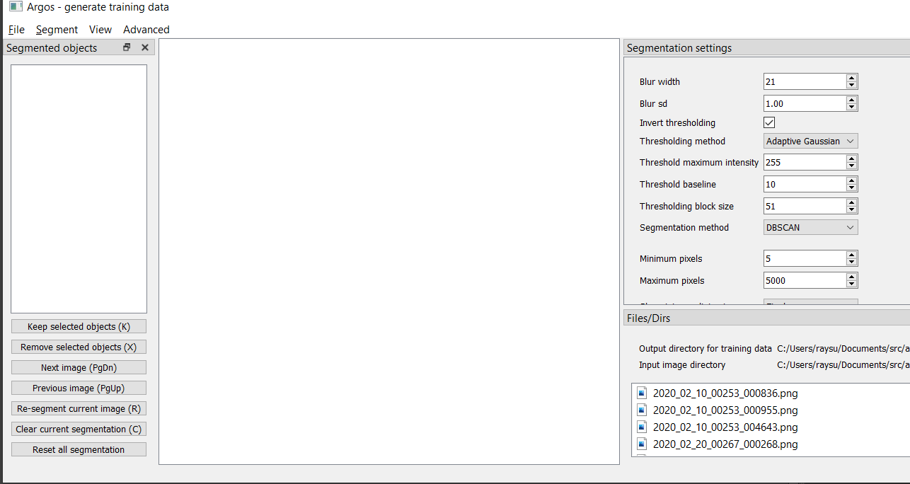
Fig. 2 Screenshot of annotate tool at startup

The Files/Dirs pane on the bottom right lists all the files in the image directory selected at startup. (Note that this pane may take up too much screen space. You can close any of the panes using the ‘x’ button on their titlebar or or move them around by dragging them with left mouse button).

The Segmentation settings pane on right allows you to choose the parameters for segmentation. See below for details on these settings.

You can press PgDn key, or click on any of the file names listed in Files/Dirs pane to start segmenting the image files. Keep pressing PgDn to go to next image, and PgUp to go back to previous image. (NOTE: On mac you may not have PgUp and PgDn keys, the equivalents are fn+UpArrow and fn+DownArrow.

It can take about a second to segment an image, depending on the image size and the method of segmentation. Once the image is segmented, the segment IDs will be listed in Segmented objects pane on the left.

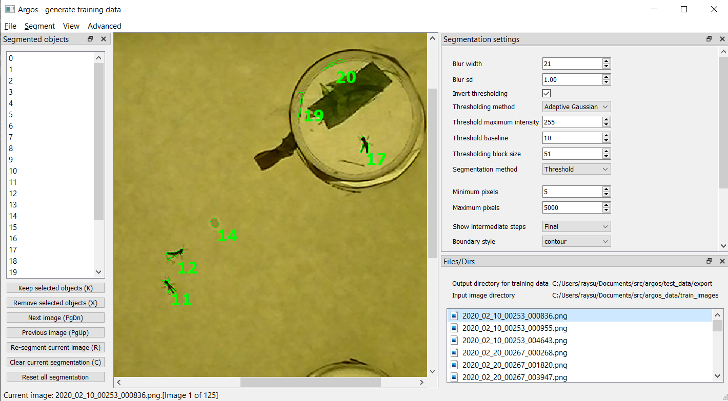
Fig. 3 Screenshot of annotate tool after segmenting an image.

The image above shows some locusts in a box with petri dishes containing paper strips. As you can see, the segmentation includes spots on the paper floor, edges of the petri dishes as well as the animals.

We want to train the YOLACT network to detect the locusts. So we must remove any segmented objects that are not locusts. To do this, click on the ID of an unwanted object on the left pane listing Segmented objects. The selected object will be outlined with dotted blue line.

You can click the Remove selected objects button on the panel at the bottom left, or press x on the keyboard to delete this segmented object.

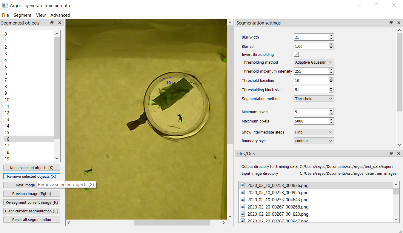
Fig. 4 Screenshot of annotate tool for selecting a segmented object. Segmented object 16 is part of the petri-dish edge and we want to exclude it from the list of annotated objects in this image.

Alternatively, if the number of animals is small compared to the spuriously segmented objects, you can select all the animals by keeping the Ctrl key pressed while left-clicking on the IDs of the animals on the left pane. Then click Keep selected objects or press k on the keyboard to delete all other segmented objects.

By default, objects are outlined with solid green line, and selected objects are outlined with dotted blue line. But you can change this from View menu.

In the View menu you can check Autocolor to make the program automatically use a different color for each object. In this case, the selected object is outlined in a thicker line of the same color, while all other object outlines are dimmed.

You can also choose Colormap from the view menu and specify the number of colors to use. Each object will be outlined in one of these colors, going back to the first color when all the colors have been used.

Segmentation settings

The segmentation settings pane allows you to control how each image is segmented. The segmentation here is done in the following steps:

1. Convert the image to gray-scale

2. Smooth the gray-scale image by Gaussian blurring. For this the following parameters can be set:

   • Blur width: diameter of the 2D Gaussian window in pixels

   • Blur sd: Standard deviation of the Gaussian curve used for blurring.

3. Threshold the blurred image. For this the following parameters can be set:

   • Invert thresholding: instead of taking the pixels above threshold value, take those below. This should be checked when the objects of interest are darker than background.

   • Thresholding method: Choice between Adaptive Gaussian and Adaptive Mean. These are the two adaptive thresholding methods provided by the OpenCV library. In practice it does not seem to matter much.

   • Threshold maximum intensity: pixel values above threshold are set to this value. It matters only for the Watershed algorithm for segmentation (see below). Otherwise, any value above the threshold baseline is fine.

   • Threshold baseline: the actual threshold value for each pixel is based on this value. When using adaptive mean, the threshold value for a pixel is the mean value in its block size neighborhood minus this baseline value. For adaptive Gaussian, the threshold value is the Gaussian-weighted sum of the values in its neighborhood minus this baseline value.

   • Thresholding block size: size of the neighborhood considered for each pixel.

   • Segmentation method: This combo box allows you to choose between several thresholding methods.

     • Threshold and Contour are essentially the same, with slight difference in speed. They both find the blobs in the thresholded image and consider them as objects.

     • Watershed uses the watershed algorithm from OpenCV library. This is good for objects covering large patches (100s of pixels) in the image, but not so good for very small objects. It is also slower than Contour/Thresholding methods.

     • DBSCAN uses the DBSCAN clustering algorithm from scikit-learn package to spatially cluster the non-zero pixels in the thresholded image. This is the slowest method, but may be good for intricate structures (for example legs of insects in an image are often missed by the other algorithms, but DBSCAN may keep them depending on the parameter settings). When you choose this method, there are additional parameters to be specified. For a better understanding of DBSCAN algorithm and relevant references see its documentation in scikit-learn package: https://scikit-learn.org/stable/modules/generated/sklearn.cluster.DBSCAN.html

       • DBSCAN minimum samples: The core points of a cluster should include these many neighbors.

       • DBSCAN epsilon: this is the neighborhood size, i.e., each core point of a cluster should have minimum samples neighbors within this radius. Experiment with it (try values like 0.1, 1, 5, etc)!

   • Minimum pixels: filter out segmented objects with fewer than these many pixels.

   • Maximum pixels: filter out segmented objects with more than these many pixels.

   • Show intermediate steps: used for debugging. Default is Final which does nothing. Other choices, Blurred, Thresholded, Segmented and Filtered show the output of the selected step in a separate window.

   • Boundary style: how to show the boundary of the objects. Default is contour, which outlines the segmented objects. bbox will show the bounding horizontal rectangles, minrect will show smallest rectangles bounding the objects at any angle, and fill will fill the contours of the objects with color.

   • Minimum width: the smaller side of the bounding rectangle of an object should be greater or equal to these many pixels.

   • Maximum width: the smaller side of the bounding rectangle of an object should be less than these many pixels.

   • Minimum length: the bigger side of the bounding rectangle of an object should be greater or equal to these many pixels.

   • Maximum length: the bigger side of the bounding rectangle of an object should be less than these many pixels.

Save segmentation

You can save all the data for currently segmented images in a file by pressing Ctrl+S on keyboard or selecting File->Save segmentation from the menu bar. This will be a Python pickle file (extension .pkl or .pickle).

Load segmentation

You can load segmentation data saved before by pressing Ctrl+O on keyboard or by selecting File->Open saved segmentation from the menu bar.

Export training and validation data

Press Ctrl+E on keyboard or select File->Export training and validation data from menubar to export the annotation data in a format that YOLACT can read for training.

This will prompt you to choose an export directory. Once that is done, it will bring up a dialog box as below for you to enter some metadata and the split of training and validation set.

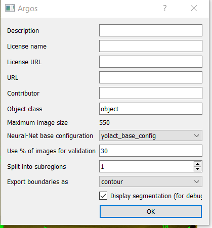
Fig. 5 Screenshot of annotate tool export annotation dialog

• Object class: here, type in the name of the objects of interest.

• Neural-Net base configuration: select the backbone neural network if you are trying something new. The default yolact_base_config should work with the pretrained resnet 101 based network that is distributd with YOLACT. Other options have not been tested much.

• Use % of images for validation: by default we do a 70-30 split of the available images. That is 70% of the images are used for training and 30% for validation.

• Split into subregions: when the image is bigger than the neural network’s input size (550x550 pixels in most cases), randomly split the image into blocks of this size, taking care to keep at least one segmented object in each block. These blocks are then saved as individual training images.

• Export boundaries as: you can choose to give the detailed contour of each segmented object, or its axis-aligned bounding rectangle, or its minimum-area rotated bounding rectangle here. Contour provides the most information.

  Once done, you will see a message titled Data saved showing the command to be used for training YOLACT. It is also copied to the clipboard, so you can just use the paste action on your operating system to run the training from a command line.

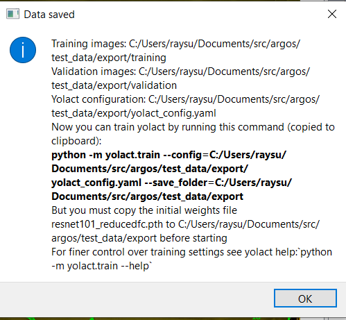
Fig. 6 Screenshot of suggested command line after exporting annotations.

Train YOLACT backbone network

After exporting the data to desired destination, you will find two folders: training and validation, and a configuration file in YAML format with the extension .yaml.

Modify this configuration file to fit your requirements. Two parameters that may need tweaking are:

• max_iter: the maximum number of training iterations in this configuration file.

• batch_size: the number of images to use in each batch of training data. If the system has multiple GPUs or large enough dedicated video memory, increasing this can make the training faster. If the training script crashes because CUDA could not allocate enough memory, then reducing this number may reduce memory requirements.

To train in the destination folder, use cd command in the command prompt to switch to this folder, create a weights folder, copy the backbone network (e.g. resnet101_reducedfc.pth for resnet101) to this folder and run the training with:

python -m yolact.train --config=yolact_config.yaml --save_folder=weights

To find out various options available in the training script, try:

python -m yolact.train -h

If you do not have a CUDA capable GPU, you can still train YOLACT on Google Colab. Here is a jupyter notebook showing how: https://github.com/subhacom/argos_tutorials/blob/main/ArgosTrainingTutorial.ipynb. You can copy this notebook to your own Google account and run it after uploading the training data generated by Argos Annotation tool. You have to select Runtime -> Change runtime type in the menu and then in the popup window choose GPU from the drop-down menu under Hardware accelerator. Note that Google automatically disconnects you after long inactivity. The script saves the intermediate trained-network and you can restart from the last saved version.

Valid backbones: YOLACT defines some configurations based on certain backbones (defined in yolact/data/config.py). These are (along with the filename for imagenet-pretrained weights): ResNet50 (resnet50-19c8e357.pth) and ResNet101 (resnet101_reducedfc.pth), and DarkNet53 (darknet53.pth). The configurations are:

• yolact_base_config: resnet101, maxsize: 550

• yolact_im400_config: resnet101, maxsize: 400

• yolact_im700_config: resnet101, maxsize: 700

• yolact_resnet50_config: resnet50, maxsize: 550

• yolact_resnet50_pascal_config: resnet50 for training with Pascal SBD dataset

When training with a custom dataset, use one of the above as base in the annotation tool when exporting training data.

Track interactively

Usage:

python -m argos_track

In Argos, this is the main tool for tracking objects automatically. Argos tracks objects in two stages, first it segments the individual objects (called instance segmentation) in a frame, and then matches the positions of these segments to that in the previous frame.

The segmentation can be done by a trained neural network via the YOLACT library, or by classical image processing algorithms. Each of these has its advantages and disadvantages.

Basic usage

This assumes you have a YOLACT network trained with images of your target object. YOLACT comes with a network pretrained with a variety of objects from the COCO database. If your target object is not included in this, you can use the Argos annotation tool (argos.annotate) to train a backbone network.

When you start Argos tracker, a window with an empty central widget is presented (Fig. 7).

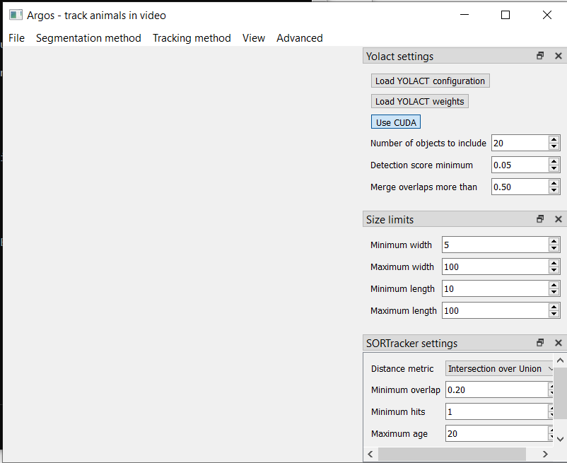
Fig. 7 Screenshot of tracking tool at startup

1. Use the File menu to open the desired video. After selecting the video file, you will be prompted to:

   1. Select output data directory/file. You have a choice of CSV (text) or HDF5 (binary) format. HDF5 is recommended.

   2. Select Yolact configuration file, go to the config directory inside argos directory and select yolact.yml.

   3. File containing trained network weights, and here you should select the babylocust_resnet101_119999_240000.pth file.

2. This will show the first frame of the video in the central widget. On the right hand side you can set some parameters for the segmentation (Fig. 8).

   

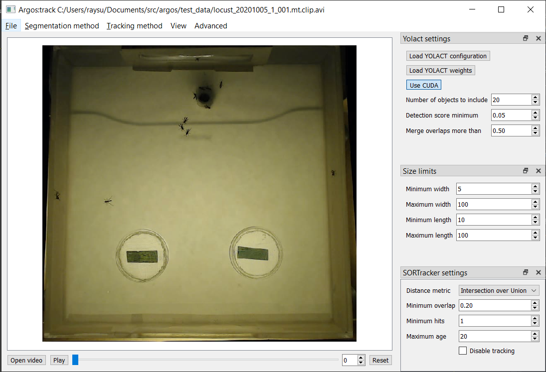
   Fig. 8 Tracking tool after loading video and YOLACT configuration and network weights.

   The top panel on the right is Yolact settings with the following fields:

   1. Number of objects to include: keep at most these many detected objects.

   2. Detection score minimum: YOLACT assigns a score between 0 and 1 to each detected object to indicate how close it is to something the network is trained to detect. By setting this value higher, you can exclude spurious detection. Set it too high, and decent detections may be rejected.

   3. Merge overlaps more than: If the bounding boxes of two

      detcted objects overlap more than this fraction of the smaller one, then consider them parts of the same object.

   The next panel, Size limits allows you to filter objects that are too big or too small. Here you can specify the minimum and maximum width and length of the bounding boxes, and any detection which does not fit will be removed.

   The bottom panel, SORTracker settings allows you to parametrize the actual tracking. SORTracker matches objects between frames by their distance. Default distance measure is Intersection over Union or IoU. This is the ratio of the area of intersection to the union of the two bounding boxes.

   • Minimum overlap: if the overlap between predicted position of an object and the actual detected position in the current frame is less than this, it is considered to be a new object. Thus, if an animal jumps from one position to a totally different position, the algorithm will think that a new object has appeared in the new location.

   • Minimum hits: to avoid spurious detections, do not believe a detected object to be real unless it is detected in this many consecutive frames.

   • Maximum age: if an object goes undetected for this many frames, remove it from the tracks, assuming it has gone out of view.

3. Start tracking: click the Play/Pause button and you should see the tracked objects with their bounding rectangles and Ids. The data will be saved in the filename you entered in step above (Fig. 9).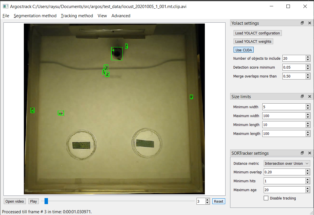

   

   Fig. 9 Tracking in progress. The bounding boxes of detected objects are outlined in green. Some spurious detections are visible which can be later corrected with the argos.review tool.

   If you choose CSV above, the bounding boxes of the segmented objects will be saved in {videofile}.seg.csv with each row containing frame-no,x,y,w,h where (x, y) is the coordinate of the top left corner of the bounding box and w and h are its width and height respectively.

   The tracks will be saved in {videofile}.trk.csv. Each row in this file contains frame-no,track-id,x,y,w,h.

   If you choose HDF5 instead, the same data will be saved in a single file compatible with the Pandas library. The segementation data will be saved in the group /segmented and tracks will be saved in the group /tracked. The actual values are in the dataset named table inside each group, with columns in same order as described above for CSV file. You can load the tracks in a Pandas data frame in python with the code fragment:

   tracks = pandas.read_hdf(tracked_filename, 'tracked')
   

Selecting a region of interest (ROI)

If you want to process only a certain part of the frames, you can draw an ROI by clicking the left mouse-button to set the vertices of a polygon. Click on the first vertex to close the polygon. If you want to cancel it half-way, click the right mouse-button.

Classical segmentation

Using the Segmentation method menu you can switch from YOLACT to classical image segmentation for detecting target objects. This method uses patterns in the pixel values in the image to detect contiguous patches. If your target objects are small but have high contrast with the background, this may give tighter bounding boxes, and thus more accurate tracking.

When this is enabled, the right panel will allow you to set the parameters. The parameters are detailed in argos.annotate.

Briefly, the classical segmentation methods work by first converting the image to gray-scale and then blurring the image so that sharp edges of objects are smoothed out. The blurred image is then thresholded using an adaptive method that adjusts the threshold value based on local intensity. Thresholding produces a binary image which is then processed to detect contiguous patches of pixels using one of the available algorithms.

Track in batch mode (non-interactively)

Usage:

python -m argos_track.batchtrack -i {input_file} -o {output_file}
-c {config_file}

Try python -m argos_track.batchtrack -h for details of command-line options.

This program allows non-interactive tracking of objects in a video. When using classical segmentation this can speed things up by utilizing multiple CPU cores.

It may be easier to use the interactive tracking argos_track to play with the segmentation parameters to see what work best for videos in a specific setting. The optimal setting can then be exported to a configuration file which will then be passed with -c command line option .

Examples

Use YOLACT for segmentation and SORT for tracking:

python -m argos_track.batchtrack -i video.avi -o video.h5 -m yolact \\
--yconfig=config/yolact.yml -w config/weights.pth -s 0.1 -k 10 \\
--overlap_thresh=0.3 --cuda=True \\
--pmin=10 --pmax=500 --wmin=5 --wmax=100 --hmin=5 --hmax=100 \\
-x 0.3 --min_hits=3 --max_age=20

The above command tells the batchtrack script to read the input video video.avi and write the output to the file video.h5. The rest of the arguments:

• -m yolact tells it to use YOLACT as the segmentation method.

• --yconfig=config/yolact.yml: Read YOLACT settings from the file config/yolact.yml

• -w config/weights.pth: Read YOLACT neural network weights from the file config/weights.pth.

• -s 0.1: Include detections with score above 0.1

• -k 10: Keep only the top 10 detections.

• --overlap_thresh=0.3: At segmentation stage, merge detections whose bounding boxes overlap more than 0.3 of their total area.

• --cuda=True: use GPU acceleration.

• --pmin=10: Include objects at least 10 pixels in bounding box area.

• --pmax=500: Include objects at most 500 pixels in bounding box area.

• --wmin=5: Include objects at least 5 pixels wide.

• --wmax=100: Include objects at most 100 pixels wide.

• --hmin=5: Include objects at least 5 pixels long.

• --hmax=100: Include objects at most 100 pixels long.

• -x 0.3: In the tracking stage, if objects in two successive frames overlap more than 0.3 times their combined area, then consider them to be the same object.

• --min_hits=3: An object must be detcted at least in 3 consecutive frames to be included in the tracks.

• --max_age=20: If an object cannot be matched to any detected object across 20 successive frames, then discard it (possibly it exited the view). [Remember that if you have a 30 frames per second video, 20 frames means 2/3 second in real time.]

All of this can be more easily set graphically in argos_track and exported into a file, which can then be passed with -c {config_file}.

Review and correct tracks

Usage:

python -m argos.review

Basic operation

At startup it will show a window with two empty panes separated in the middle by three empty lists titled Previous tracks, All tracks and Current tracks like Fig. 10 below.

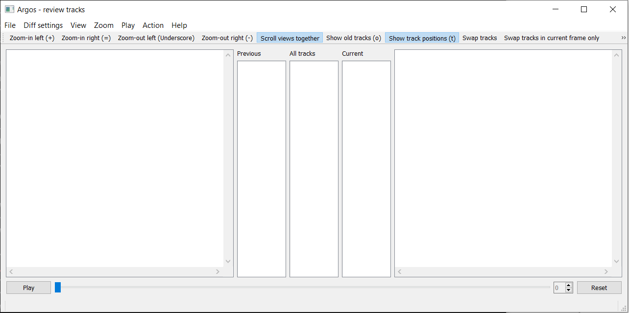
Fig. 10 Screenshot of review tool at startup

To start reviewing tracked data, select File->Open tracked data from the menubar or press Ctrl+O on keyboard. This will prompt you to pick a data file. Once you select the data file, it will then prompt you to select the corresponding video file. Once done, you should see the first frame of the video on the right pane with the bounding boxes (referred to as bbox for short) and IDs of the tracked objects (Fig. 11).

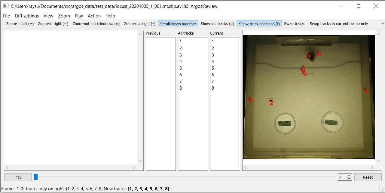
Fig. 11 Screenshot of review tool after loading data

Here you notice that trackid 4 is spurious. So you select it by clicking on the entry in Right tracks list. As you select the enetry, its bbox and ID on the image change color (and line style) (Fig. 12). If the Show track position button is checked, like in the screenshot, then you will also see the path this ID takes in color turning from dark purple at the start to light yellow at the end. Note that this path only takes into account what is already saved in the file, and not any unsaved changes you made to the track ID. In order to update the path to include all the changes you made, save the data file first.

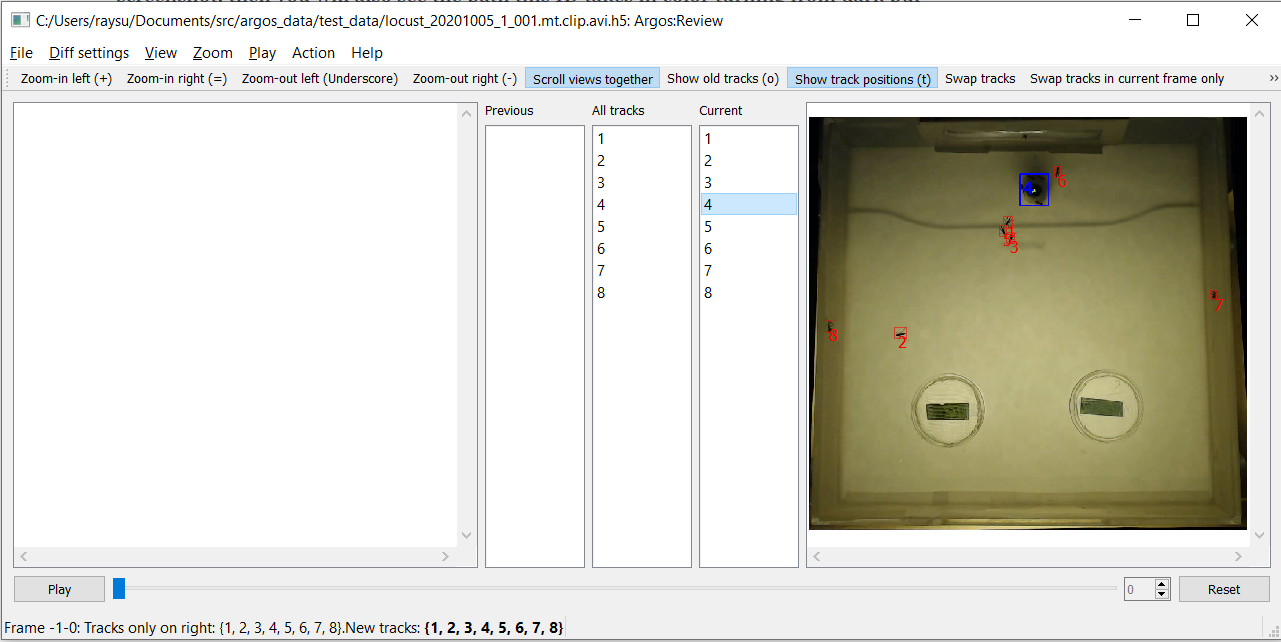
Fig. 12 Screenshot of review tool after selecting object

Now delete object 4 by pressing x or Delete on keyboard, or selecting Delete track from Action in menubar (Fig. 13). On MacOS, the delete key is actually backspace, and you have to use fn+delete to delete an object.

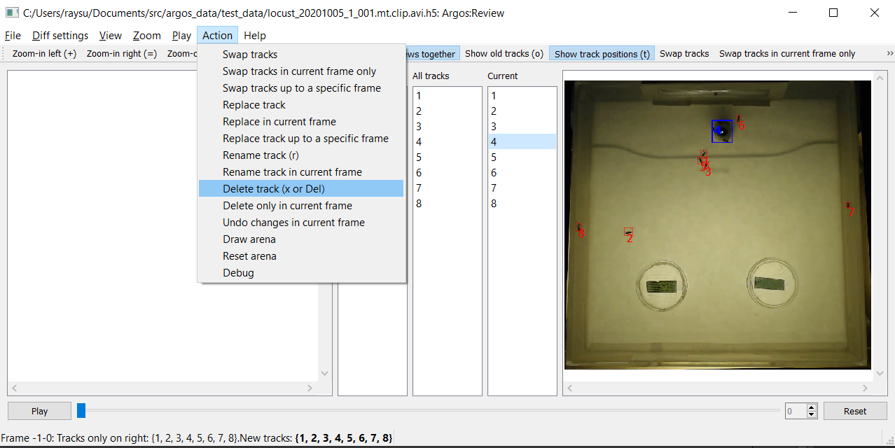
Fig. 13 Screenshot of review tool deleting object

Once you delete 4, selection will change to the next object (# 5) and the path taken by it over time will be displayed in the same purple-to-yellow color code (Fig. 14) 1. Also notice that the window title now has a * before it, indicating that you have unsaved changes.

1

Changing the frame will clear the selection and the path display. If you want the selection (and the path-display of the selected ID) to be retained across frames, check the menu item View->Retain selection across frames.

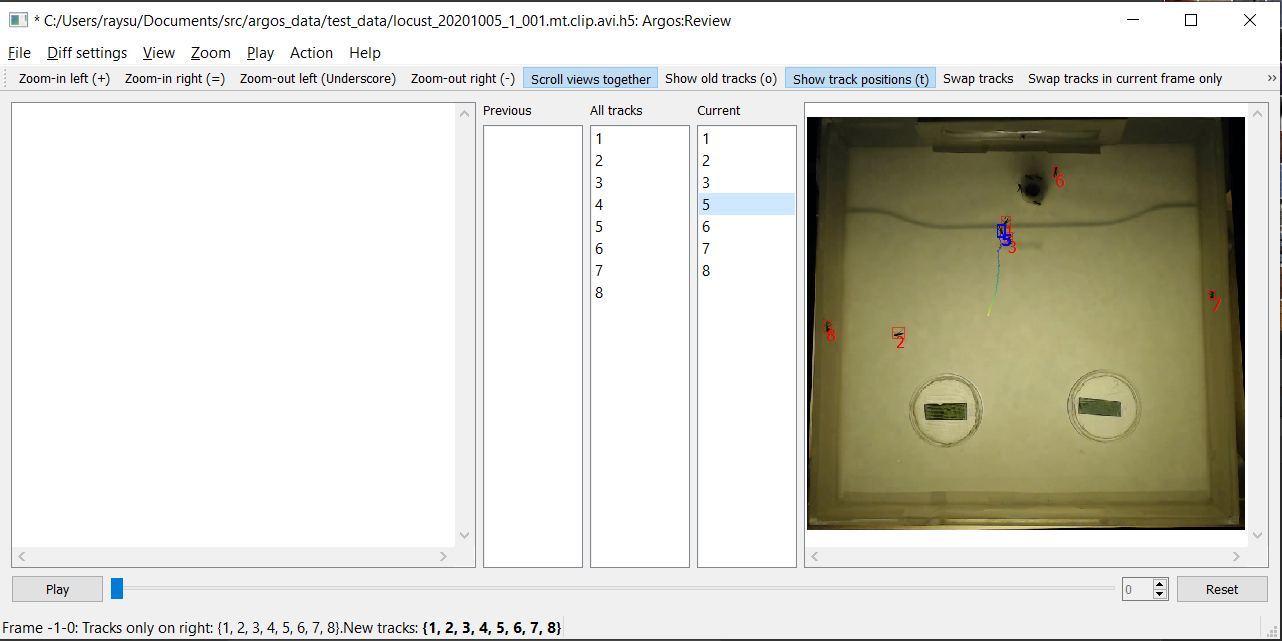
Fig. 14 Screenshot of review tool after deleting object, as the next object is selected.

Now to play the video, click the play button at bottom (or press Space bar on the keyboard). The right frame will be transferred to the left pane, and the next frame will appear in the right pane.

You will notice the spinbox on bottom right updates the current frame number as we go forward in the video. Instead of playing the video, you can also move one frame at a time by clicking the up-arrow in the spinbox, or by pressing PgDn on keyboard (fn+DownArrow on mac).

It is useful to pause and inspect the tracks whenever a new object is dected. In order to pause the video when there is a new trackid, check the Show popup message for new tracks item in the Diff settings menu (Fig. 15).

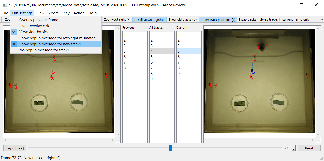
Fig. 15 Enable popup message when a new trackid appears

If you you already played through the video, then all trackids are old. In order to go back to a prestine state, click the Reset button at bottom right. If you play the video now, as soon as a new track appears, the video will pause and a popup message will tell you the new tracks that appeared between the last frame and the current frame (Fig. 16).

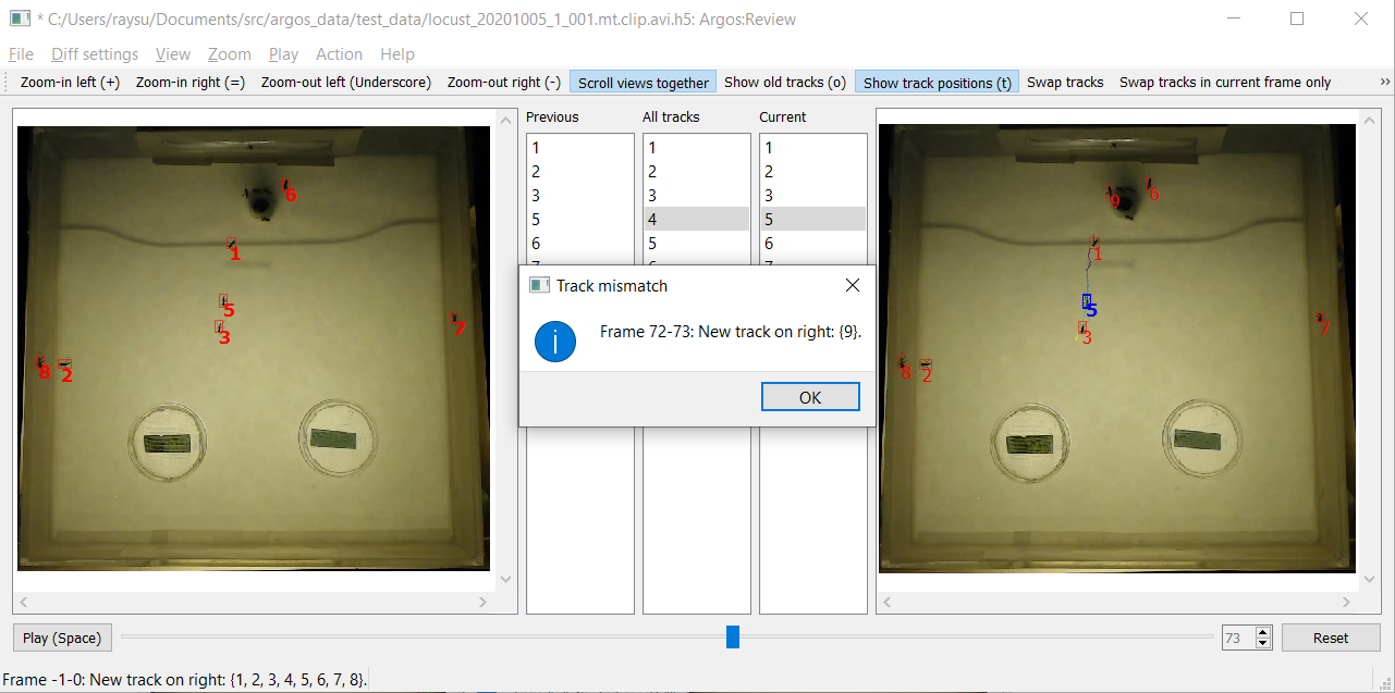
Fig. 16 Popup message when a new trackid appears

After you click OK to dispose of the popup window, the status message will remind you of the last change (Fig. 17).

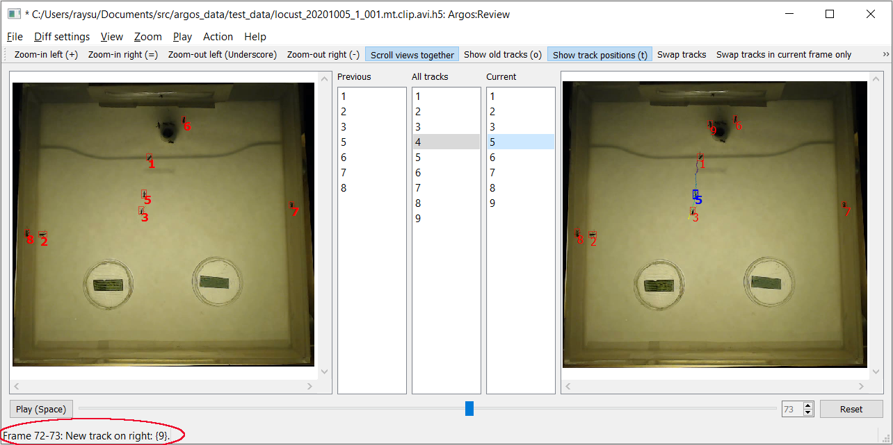
Fig. 17 Status message after a new trackid appears

You can also choose Show popup message for left/right mismatch in the Diff settings menu. In this case whenever the trackids on the previous frame are different from those on the current frame, the video will be paused with a popup message.

If you want to just watch the video without interruption, select No popup message for tracks. Whenever there is a left-right mismatch, there will still be a status message so that you can see the what and where of the last mismatch.

The other option Overlay previous frame, if selected, will overlay the previous frame on the right pane in a different color. This may be helpful for looking at differences between the two frames if the left and right display is not good enough (Fig. 18).

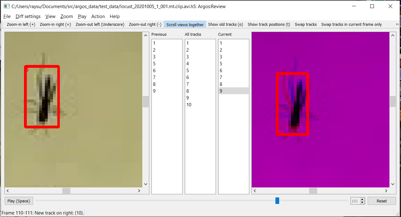
Fig. 18 Overlaid previous and current frame. The previous frame is in the red channel and the current frame in the blue channel, thus producing shades of magenta where they have similar values, and more red or blue in pixels where they mismatch.

The default view showing the previous and the current frame side by side can result in rather small area for each side. You can dedicate the entire visualization area to the current frame by turning off side-by-side view from the Diff settings menu (Fig. 19).

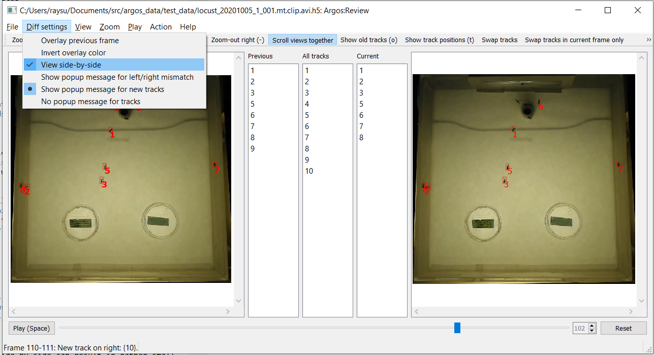
Fig. 19 Menu option to switch between side-by-side view and single-frame view.

This will keep the three lists, but remove the previous frame view (Fig. 20). A drawback of this is that now you can see the path for objects only in the current frame. But you can quickly go back and forth in frames by pressing the PgUp and PgDn keys.

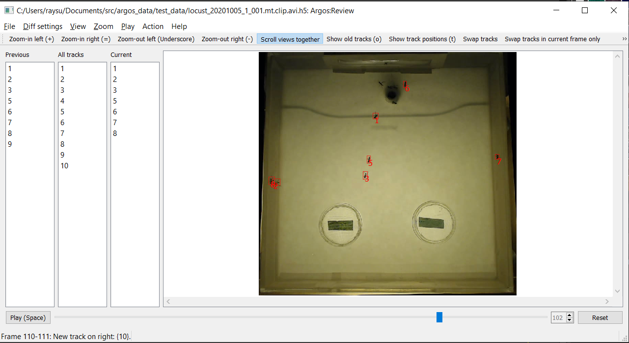
Fig. 20 Turning off side-by-side view gives the maximum screen area to the current frame, allowing closer inspection of the video.

Selecting a region of interest (ROI)

It can be tricky to fit the behavioral arena perfectly inside the camera frame. Thus one may end up including some area outside the arena when recording behavior videos. This can include clutter that is incorrectly identified as objects by the Argos Tracking tool. To exclude anything detcted outside your region of interest (ROI), you can draw a polygon to outline the ROI. To do this, first enable ROI selection mode by checking the Action->Draw arena item in the menubar (Fig. 21). Then click left mouse-button at desired vertex positions in the frame to draw a polygon that best reflects your desired region. Click on the first vertex to close the polygon. If you want to cancel it half-way, click the right mouse-button.

When finished, you can uncheck the Draw arena menu item to avoid unintended edits. When you save the corrected data, all IDs outside the arena will be excluded for all frames starting with the one on which you drew the arena.

To reset the ROI to the full frame, click Reset arena in the Action menu.

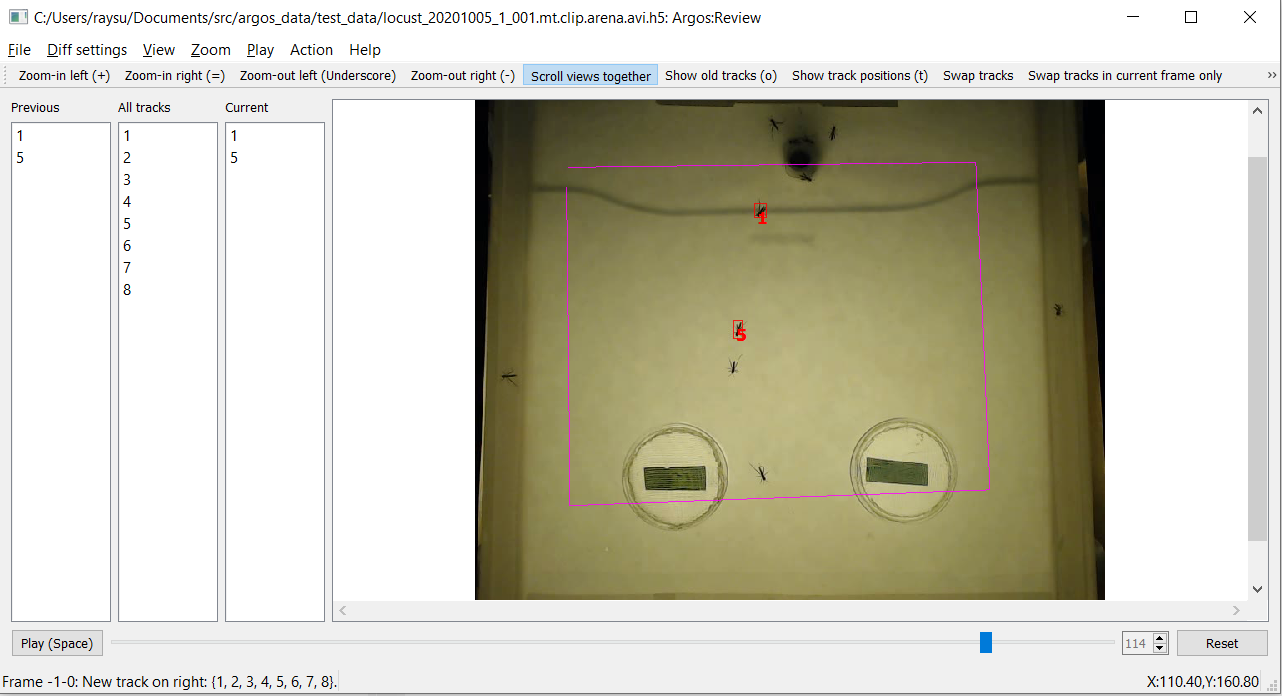
Fig. 21 Drawing a polygon (magenta lines) to specify the arena/region of interest to include only objects detected (partially) within this area.

The track lists

The three lists between the left (previous) and right (current) video frame in the GUI present the track Ids of the detected objects. These allow you to display the tracks and carry out modifications of the tracks described later).

• Previous tracks shows the tracks detected in the left (previous) frame. If you select an entry here, its detected track across frames will be overlayed on the previous frame in the left pane (Fig. 22).

• All tracks in the middle shows all the tracks seen so far (including those that have been lost in the previous or the current frame). If you select an entry here, its detected track across frames will be overlayed on the previous frame in the left pane. If you select different entries in Left tracks and All tracks, the last selected track will be displayed.

• Current tracks shows the tracks detected in the current frame (on the right). If you select an entry here, its detected track across frames will be overlayed on the current frame in the right pane.

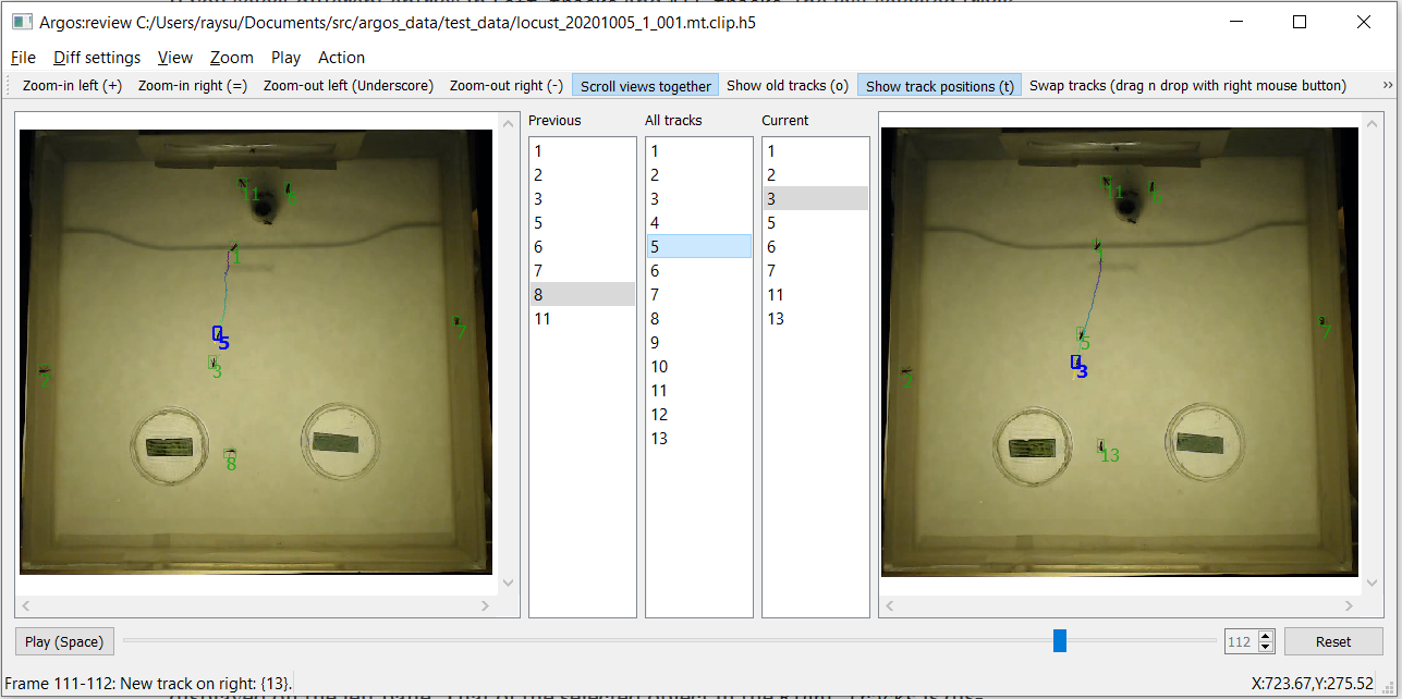
Fig. 22 The track of the selected object (track Id) in Previous tracks or All tracks is displayed on the left pane. That of the selected object in the Current tracks is displayed on the right pane.

Moving around and break points

To speed up navigation of tracked data, Argos review tool provides several shortcuts. The corresponding actions are also available in the Play menu. To play the video, or to stop a video that is already playing, press the Space bar on keyboard. You can try to double the play speed by pressing Ctrl + Up Arrow and halve the speed by pressing Ctrl + Down Arrow. The maximum speed is limited by the time needed to read and display a frame.

Instead of going through the entire video, you can jump to the next frame where a new trackid was introduced, press N key (Jump to next new track).

You can jump forward 10 frames by pressing Ctrl + PgDn and backward by pressing Ctrl + PgUp on the keyboard (the mac equivalents are command+fn+DownArrow and command+fn+UpArrow).

To jump to a specific frame number, press G (Go to frame) and enter the frame number in the dialog box that pops up.

To remember the current location (frame number) in the video, you can press Ctrl+B (Set breakpoint at current frame) to set a breakpoint. You can go to other parts of the video and jump back to this location by pressing J (Jump to breakpoint frame). To clear the breakpoint, press Shift+J (Clear frame breakpoint).

You can set a breakpoint on the appearance of a particular trackid using Set breakpoint on appearance (keyboard A), and entering the track id in the dialog box. When playing the video, it will pause on the frame where this trackid appears next. Similarly you can set breakpoint on disappearance of a trackid using Set breakpoint on disappearance (keyboard D). You can clear these breakpoints by pressing Shift + A and Shift + D keys respectively.

Finally, if you made any changes (assign, swap, or delete tracks), then you can jump to the frame corresponding to the next change (after current frame) by pressing C and to the last change (before current frame) by pressing Shift + C on the keyboard.

Correcting tracks

Corrections made in a frame apply to all future frames, unless an operation is for current-frame only. The past frames are not affected by the changes. You can undo all changes made in a frame by pressing Ctrl+z when visiting that frame.

• Deleting

  You already saw that one can delete spurious tracks by selecting it on the Right tracks list and delete it with x or Delete key. On macos, the delete key is actually backspace, and you have to use fn+delete to delete an object.

  To delete a track only in the current frame, but to keep future occurrences intact, press Shift+X instead.

  To apply this from the current frame till a specific frame, press Alt+X. A dialog box will appear so you can specify the end frame.

• Replacing/Assigning

  Now for example, you can see at frame 111, what has been marked as 12 was originally animal 5, which happened to jump from the left wall of the arena to its middle (For this I had to actually press PgUp to go backwards in the video, keeping an eye on this animal, until I could be sure where it appeared from). To correct the new trackid, we need to assign 5 to track id 12.

  The easiest way to do this is to use the left mouse button to drag the entry 5 from either the Previous tracks list or the All tracks list and drop it on entry 12 in the Right tracks list. You can also select 5 in the left or the middle list and 12 in the right list and then select Replace track from the Action menu.

  To apply this only in the current frame keep the Shift key pressed while drag-n-dropping.

  To apply this from the current frame till a specific frame, keep the Alt key pressed while drag-n-dropping. A dialog box will appear so you can specify the end frame.

• Swapping

  In some cases, especially when one object crosses over another, the automatic algorithm can confuse their Ids. You can correct this by swapping them.

  To do this, use the right mouse button to drag and drop one entry from the All tracks or Previous tracks list on the other in the Current tracks list. You can also select the track Ids in the lists and then click the Swap tracks entry in the Action menu.

  To apply this only in the current frame keep the Shift key pressed while drag-n-dropping.

  To apply this from the current frame till a specific frame, keep the Alt key pressed while drag-n-dropping. A dialog box will appear so you can specify the end frame.

• Renaming

  To rename a track with a different, nonexistent Id, select the track in one of the Current tracks list and then press the R key, or use the Action menu to get a prompt for the new Id number.

  To apply this only in the current frame keep the Shift key pressed while drag-n-dropping.

  To apply this from the current frame until a specific frame, keep the Alt key pressed while drag-n-dropping and specify the last frame (inclusive) in the popup dialog.

  Argos does not use negative track Id numbers, so to rename a track temporarily it is safe to use negative numbers as they will not conflict with any existing track numbers.

  Try not to use small positive integers unless you are sure that this number does not come up later as an ID. This will result in two different objects getting assigned the same ID, and thus erroneous tracks. Since the Track utility assigns IDs as positive integers in increasing order, you can also avoid ID collisions by using very large positive integers when renaming.

  Sometimes an object may be lost and found later and assigned a new ID. In this case renaming it to its original ID is equivalent to assigning (see above) the original ID.

All these actions, however, are not immediately made permanent. This allows you to undo changes that have been made by mistake. You can see the list of changes you suggested by selecting Show list of changes in the view menu, or by using the Alt+C keyboard shortcut (Fig. 23). To undo a change, go to the frame on which it was suggested, and press Ctrl+Z, or select Undo changes in current frame in the Action menu. If you made multiple changes in this frame, this operation will revert all of them.

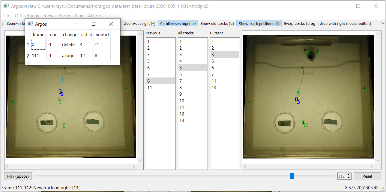
Fig. 23 List of changes to be applied to the tracks. The first entry when applied will delete the track Id 8 from frame # 24 onwards. The last entry will assign the Id 5 to the track 12 in all frames from frame # 111 onwards.

You can save the list of changes into a text file with comma separated values and load them later using entries in the File menu. The changes will become permanent once you save the data (File->Save reviewed data). However, the resulting HDF5 file will include the list of changes in a time-stamped table: changes/changelist_YYYYmmdd_HHMMSS, so you can refer back to past changes applied to the data (see Note on data format).

Finally, here are some videos showing examples of track correction using Argos Review tool: https://youtube.com/playlist?list=PLdh_edYAAElVLiBgBnLLKZY8VflMm1-LU

Tips

Swapping and assigning on the same trackid within a single frame can be problematic. Sometimes the tracking algorithm can temporarily mislabel tracks. For example, object A (ID=1) crosses over object B (ID=2) and after the crossover object A got new label as ID=3, and object B got mislabelled as ID=1. The best order of action here is to

1. swap 3 and 1, and then

2. assign 2 to 3.

This is because sometimes the label of B gets fixed automatically by the algorithm after a couple of frames. Since the swap is applied first, B’s 3 becomes 1, but there is no 1 to be switched to 3, thus there is no trackid 3 in the tracks list, and the assignment does not happen, and A remains 2. Had we first done the assignment and then the swap, B will get the label 2 from the assignment first, and as A also has label 2, both of them will become 1 after the swap.

Sometimes this may not be obvious because the IDs may be lost for a few frames and later one of the objects re-identified with the old ID of the other one.

For example this sequence of events may occur:

1. A(1) approaches B(2).

2. B(2) Id is lost

3. Both A and B get single bounding box with ID 1.

4. A gets new ID 3. B is lost.

5. A has new ID 3, B reappears with 1.

Action sequence to fix this:

1. Go back where A and B have single ID 1.

2. Swap 2 and 1.

3. Go forward when 3 appears on A.

4. Assign 1 to B.

Swapping IDs multiple times can build-up into-hard-to-fix switches between IDs, as all the changes in the change list buffer are applied to all future frames. This can be avoided by saving the data between swaps. This will consolidate all suggested changes in the buffer and clear the change list.

After swapping two IDs you may notice that one ID keeps jumping between the two animals. Even if you do the swap again when this happens in later frame, the IDs keep switching back and forth. In such a case try doing a temporary swap, i.e., a swap that applies to the current frame only.

Whenever there are multiple animals getting too close to each other, a good approach is to put a breakpoint when the algorithm confuses them for the first time, and slowly go forward several frames to figure out what the stable IDs become. Also check how long-lived these IDs are (if a new ID is lost after a few frames, it may be less work to just delete it, and interpolate the position in between). Then go back and make the appropriate changes. Remember that the path history uses the original data read from the track file and does not take into account any changes you made during a session. To show the updated path, you have to first save the data so that all your changes are consolidated.

Note on video format

Argos capture utility records video in MJPG format in an AVI container. This is available by default in OpenCV. Although OpenCV can read many video formats via the ffmpeg library, most common video formats are designed for playing sequentially, and jumping back and forth (seek) by arbitrary number of frames is not easy.

With such videos, attempt to jump frames will result in error, and the review tool will disable seek when it detects this. To enable seek when the video format permits it, uncheck the Disable seek item in the Play menu.

Note on data format

Argos saves and reads data in comma separated values in text format (.csv), and HDF5 (.h5, .hdf) format. The HDF5 format is recommended as it allows meta information, and keeps all the data together.

The HDF5 data is saved and read as Pandas DataFrame in Python under the name /tracked for track data and /segmented for raw instance segmentation. You can read these into Pandas DataFrames as pd.read_hdf(filename, ‘tracked’) and pd.read_hdf(filename, ‘segmented’) respectively (assuming you first imported pandas with import pandas as pd).

The tracked dataframe has these columns: frame, trackid, x, y, w, h where frame is the video frame number, trackid is a non-negative integer identifying a track, x, y, w, h describe bounding box of the tracked object in this frame where (x, y) is the coordinate of top left corner of the bounding box, w its width and x its height.

In addition, when you make changes in the Review tool, it saves the changes you made in the group changes. There will be a subgroup for each save with its timestamp, and you can load these as Pandas DataFrames. The timestamp informs you about when each set of changes was saved, i.e., the order of operations. Here is a code snippet demonstrating how you can check the changes:

import pandas as pd

fd = pd.HDFStore('mytrackfile.h5', 'r')

for ch in fd.walk('/changes'):  # traverse recursively under this group
    print('#', ch)              # this prints a single line
    change_nodes = ch[-1]       # the last entry is the list of leaf nodes
    for node in change_nodes:   # go through each changelist
        changelist = fd[f'/changes/{node}']   # recover the changes
        print(node)
        print(changelist)
fd.close()

This shows something like the following:

  # ('/changes', [], ['changelist_20211102_055038', 'changelist_20211102_070504'])
  changelist_20211102_055038
      frame  end     change  code  orig  new  idx
  0      68   -1  op_delete     5     2   -1    0
  1     150   -1  op_assign     3     6    1    1
  2     250   -1  op_assign     3     9    8    2
  3     273   -1  op_assign     3    10    8    3
  4     508   -1  op_delete     5    11   -1    4
  5     679   -1  op_assign     3    12    8    5
  6     740  746  op_assign     3     8   16    8
  7     745   -1  op_assign     3    14    5    6
  8     757   -1  op_assign     3    16    8    7
  9     768   -1  op_assign     3    17   16    9
  10    772   -1  op_assign     3    20    8   10
  11    811   -1  op_assign     3    21    5   11
  12    823   -1  op_assign     3    22   19   12
  13    889   -1  op_assign     3    23    5   13
  changelist_20211102_070504
       frame  end     change  code  orig  new  idx
  0      888   -1  op_delete     5    23   -1    1
  1      923   -1  op_assign     3    24    7    0
  2      956   -1  op_assign     3    25    7    2
  3     1043   -1  op_assign     3    26    5    3
  4     1045   -1  op_assign     3    28    5    4
  ..     ...  ...        ...   ...   ...  ...  ...
  122   9037   -1  op_assign     3   127   16  123

[127 rows x 7 columns]

This shows that we saved change lists at two time points. For each, the first column is just the pandas dataframe index, then we have the frame number from which this change was applied. The end column specifies the frame till which (inclusive) this change was applied. An entry of -1 indicates the end is the last frame of the video. The change column specifies a string describing the change, and code the numeric code for the same. orig specifies the original ID and new the new ID. In case of delete operation, the new ID is -1. Finally, the last columns, idx specifies an index to maintain the order in which the operations were specified by the user.

Utility to display the tracks

Usage:

python -m argos.plot_tracks -v {videofile} -f {trackfile} \\
--torig {original-timestamps-file} \\
--tmt {motiontracked-timestamps-file} \\
--fplot {plotfile} \\
--vout {video-output-file}

Try python -m argos.plot_tracks -h for a listing of all the command line options.

This program allows displaying the (possibly motion-tracked) video with the bounding boxes and IDs of the tracked objects overlaid. Finally, it plots the tracks over time, possibly on a frame of the video.

With --torig and --tmt options it will try to read the timestamps from these files, which should have comma separated values (.csv) with the columns inframe, outframe, timestamp (If you use :py:module:argos.capture to capture video, these will be aleady generated for you). The frame-timestamp will be displayed on each frame in the video. It will also be color-coded in the plot by default.

With the --fplot option, it will save the plot in the filename passed after it.

With the --vout option, it will save the video with bounding boxes in the filename passed after it.

With --trail option, it will show the trail of each animal from the past trail frames. However, if trail_sec flag is set, it will show the trails for past trail seconds.

With --randcolor flag set, it will draw each track (bbox and ID) in a random color.

Summary of keyboard shortcuts

Note

On mac notebooks, Ctrl = command, Alt = option, PgUp = fn + up-arrow, PdDn = fn + down-arrow, Delete = fn + delete.

The equivalent of PC keys are listed here: https://support.apple.com/guide/mac-help/windows-keys-on-a-mac-keyboard-cpmh0152/mac

Table 1 Keyboard shortcuts for Annotation tool

Keys	Action
+	Zoom-in
-	Zoom-out
PgDn (mac: fn + down-arrow)	Next image
PgUp (mac: fn + up-arrow)	Previous image
Delete (mac: fn + delete)	Remove segmentation
x	Remove selected segmentations
k	Keep selected segmentations (delete unselected)
Shift + x	Keep selected segmentations (delete unselected)
c	Clear segementation of current image
r	Segment current image again
Ctrl + s	Save segmentation to file
Ctrl + o	Load segementation from file
Ctrl + e	Export annotated data as training and validation sets in COCO format

Table 2 Keyboard shortcuts for Tracking tool

Keys	Action
Spacebar	Play -> Pause, Pause -> Play, OK in popup dialogs
Ctrl + o	Open video

Table 3 Keyboard shortcuts for Review tool

Keys	Action
Ctrl + o	Open tracks and video file
Ctrl + s (mac: command + s)	Save reviewed tracks
Spacebar	Play-> Pause, Pause -> Play
b	Set breakpoint
Ctrl + b	Set breakpoint at current frame
Shift + b	Clear breakpoint
a	Set breakpoint at apparance of an ID
d	Set breakpoint at disappearance of an ID
Shift + a	Clear breakpoint at appearance of an ID
Shift + d	Clear breakpoint at disappearance of an ID
g	Go to frame
j	Jump to frame with breakpoint
PgDn (mac: fn + down-arrow)	Go to next frame
PgUp (mac: fn + up-arrow)	Go to previous frame
Ctrl + PgDn (mac: command + fn + down-arrow)	Jump 10 frames forward
Ctrl + PgUp (mac: command + fn + up-arrow)	Jump 10 frames back
n	Jump to next mismatch of IDs between two successive frames
p	Jump to previous mismatch of IDs between two successive frames
c	Jump to next change in ChangeList from current frame
Shift + c	Jump to last change in ChangeList from current frame
+	Zoom-in previous frame
_ (underscore)	Zoom-out previous frame
=	Zoom-in current frame
- (minus)	Zoom-out current frame
o	Toggle display of old tracks (ghosted)
t	Toggle display of path history of tracks
s	Toggle retaining selection across change of frames
Alt + c (twice if window is hidden)	Show list of changes
x	Delete selected ID
Delete (mac: fn + delete)	Delete selected ID from current and future frames
Shift + x	delete selected ID in current frame only
Shift + Delete (mac: Shift + fn + delete)	delete selected ID in current frame only
Alt + x (mac: option + x)	Delete selected ID from a range of frames
Alt + delete (mac: option + fn + delete)	Delete selected ID from a range of frames
r	Rename selected track
Shift + r	Rename selected track only in current frame
Ctrl + z	Undo changes in current frame
Ctrl + PgUp (mac: command + fn + up-arrow)	Increase the speed of playback
Ctrl + PgDn (mac: command + fn + down-arrow)	Decrease the speed of playback
Shift + Mouse Wheel Down	Go to next frame
Shift + Mouse Wheel Up	Go to previous frame
Shift + Ctrl + Mouse Wheel Down	Go forward 10 frames
Shift + Ctrl + Mouse Wheel Up	Go backward 10 frames
Ctrl + Mouse Wheel Down	Zoom out
Ctrl + Mouse Wheel Up	Zoom in